Aperture Photometry with MaximDL
Learn to measure the perceived brightness of astronomical objects and perform a time-series analysis
What is photometry?
Photometry, as the name implies, is the measurement (-metry, metriā) of light (photo-, phôs) radiated by astronomical objects. More specifically, photometry is the science of measuring perceived brightness of an object to the human eye. There are various ways that photometry can be performed, but in this tutorial, we will be focusing solely on the simpliest technique: aperture photometry.
Aperture photometry consists of two parts:
- summing of pixel counts in a circular area, also known as an aperture, centred on a point source (a star, an asteriod, or a supernova), and
- subtracting the excess unwanted pixels that are contributed from sources behind and in front of the object.
The excess pixels in (2) are also known as sky or background, and we will use these two terms interchangeably.
When you are doing aperture photometry (from a GUI, at least), you will see something like the following. Aperture photometry basically sums the counts in the “aperture” area and subtracting the mean noise in the background defined in the “sky annulus” area:
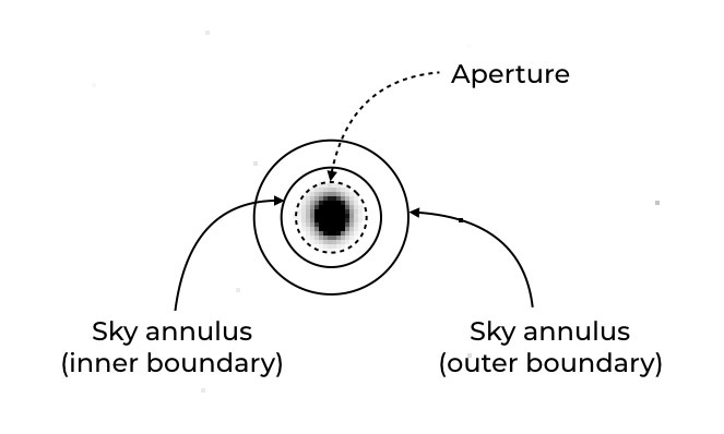
You will see an almost identical illustration with MaxIm DL later.
What’s MaxIm DL?
MaxIm DL is a powerful astronomy imaging software that has a user-friendly GUI. Until recently, it was one of the greatest mysteries in the Universe as to what “MaxIm” stands for. There is a massive list of functions that one can use MaxIm DL for, such as operating CCD cameras and controlling filter wheels and guiders. For our purpose, we will be primarily using MaxIm’s image processing and analysis features, particularly its photometry tool.
Using MaxIm DL’s Photometry Function
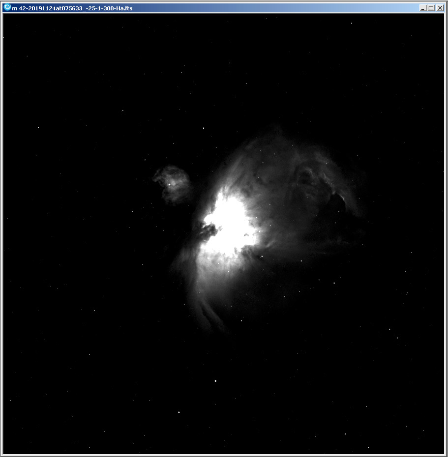
You can use the photometry function on any object as long as the object that you’re looking at is a point source. To begin, we will be using an H-alpha image of the Orion Nebula (M42).
Open the file and you should see a white-and-black of the Orion Nebula.
I will pick an arbitrary point source to photometer—this one right here:

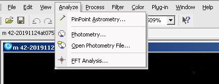
To begin our photometry, go to Analyze > Photometry:
Mouse your aperture tool over the object that you want to photometer. Right-click to adjust the aperture radius, gap width, and annulus thickness accordingly till you see something like the following:
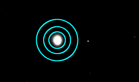
The principle is that the aperture should cover the point source tightly, with no spillover and as little black space as possible.
Once you have moused the aperture tool over the object perfectly, you can double click the moused-over area to lock it. You can see the statistics in the given window on the object. The image below explains what each value means:
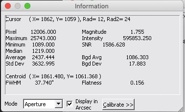
To calculate the magnitude of the point source, use the following formula:

Where m is the magnitude of the source,
ADU (Analog-to-Digital Unit) is the intensity, and
t the exposure time (s) of the image.
The figure you get from the above, however, is not the apparent magnitude of the object, but the instrument magnitude. To obtain the apparent magnitude, we have to figure out the offset of the telescope at the Nieves Observatory, also known as the zero point. That will be a topic I’ll add to this tutorial when I have more time. Let’s perform some time-series photometry!
Time series observation with XO-6b
Measuring the brightness of a stable and unchanging star is not an exciting thing to do. The data that you obtain do not give you much information about the object, apart from its brightness and possibly temperature. A more interesting use of photometry is in transient astronomy, where we measure the change in brightness of a fast-evolving object—a transient—over the span of months, weeks, days, or even hours. These transients could be astronomical objects going through rapid changes, such as a pulsing red giant, or something as mundane as an exoplanet moving across its host star from our line of sight.
As the brightness of the transient changes rather quickly, we can create a light curve from our time-series observation to show the change of the object’s brightness over time. We will create a time series in this tutorial using an exoplanet transit as an example.
A transit is an astronomical phenomenon when an exoplanet obscures part of the light from its host star to our line of sight as it orbits around the host star. We should be expecting a dip in our light curve in our own measurement. Here’s an illustration of the mechanics behind the phenomenon:

Download the folder of 160 images of an exoplanet transiting its host star, taken with the Nieves Observatory in Jan 2020.
(Warning, file size: 5.0GB)
Differential photometry
The technique that we are using for a time series is a subset of aperture photometry known as differential photometry. In differential photometry, we will photometer at least two sources at once in a single image. The first object is our object of interest, while the other is a reference object/star. To get the resulting differential magnitude, we simply subtract the reference’s magnitude from the object’s magnitude:

Why can’t we simply use the magnitude of the object (m_object)? Reason being: We do not know for sure if the object of interest is a transient, and any variation of the object’s magnitude over time could be caused by other factors, such as varying night-to-night weather conditions, rather than a real change in the object’s brightness. Since both the object and the reference star are observed at the same time, with the same filters, using the same instrument, the observational variables are cancelled out when we obtain the differential magnitude.
Let’s now begin with the photometry:
- Go to Analyze > Photometry
- Click on “Add Files…”
- Navigate to the folder with the 160 images of XO-6b, and select all
- Expand the folder with the “+” sign, and click on the first file listed
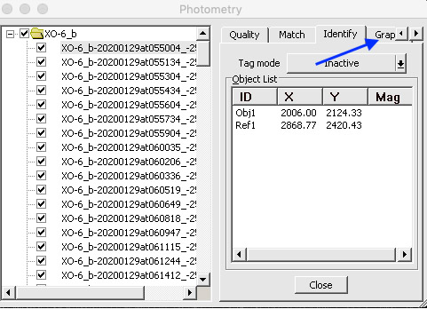
- Click on the “Identify” tab on the Photometry window
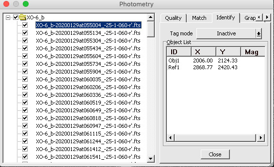
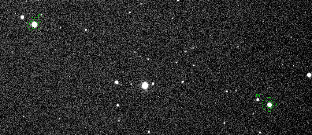
You will see the first image of the series on your screen. XO-6, the object that we are studying, is somewhere in the centre of the image. Mouse your aperture over the object, and remember to adjust the aperture size, gap width, and annulus thickness accordingly. Once all of those are perfect, right-click and click on “Tag New Object”. An identifier will circle the object and label it as “Obj1”.
Next, we select our reference star. While we can have as many reference stars as we like, we are only using one for now. The reference star should have the following characteristics:
- They should be about the same brightness as the object of interest
- They should not be saturated/overexposed
- They should have similar FWHM
- They should not be corrupted by other sources in their vicinity
I have selected one that is not too far away from XO-6 which satisfies all of the above conditions. Right-click to designate as a reference star. It should automatically label the reference star as “Ref1”.
Obtaining the light curve
Once you’ve set the object and reference, MaxIm DL can automatically photometer every single image in the folder and produce a light curve once its done with the automatic photometry. To do so, click on the “Graph” tab on the Photometry window.
You will notice that there’s nothing on the graph. Ideally, this should not happen, but because the quality of our imaging of the object may not be consistent (clouds come and go throughout the night), some of the photometry is performed imperfectly. We will have to manually correct the photometry that are not properly done.
To do so, we will have to check every single image in the photometry window. Go through 1 to 160. You will find that the aperture tool is calibrated wrongly for some images. Drag it back to the centre of the source.
Do this for all of the images, and slowly you’ll see some points on the graph. Eventually, you’ll get the following. (If you don’t, right-click the y-axis of the graph and click “Auto”.)
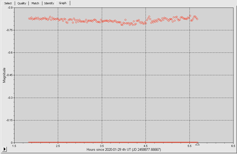
The graph is plotting the (instrumental) brightness of both the exoplanet star and the reference star. Dips in transits are extremely small, and so we have to zoom into the graph to see the dip in the light curve properly. We can ignore the data of the reference star.
To adjust the graph to show the dip clearer, right-click the y-axis and set:
- “Faintest…” to -0.75 magnitudes
- “Brightest…” to -0.9 magnitudes
You should see the following light curve:
Can you spot the transit?